Adding Data to an ArcView Project: JOINing tables
We have a list of Analytical Variables derived from the 1990 Census data. Some are easily constructed by "normalizing" one variable with another, as we did by dividing total population by household to yield a figure for each county of "mean household size". But some of these Analytical Variables require more calculation than ArcView will happily do [though ArcView's Field Calculator is pretty powerful --a subject for another exercise, perhaps], and the easiest way to derive such Analytical Variables is [arguably] to use Excel to execute the formulas and then JOIN the resulting .dbf table to an existing ArcView Theme Table.
This exercise doesn't take you through the messiness of Excel --I've already calculated a number of the Analytical Variables and saved them in a .dbf file for you to manipulate. Here's the procedure for today's adventure (once again, follow the steps carefully...):
- Launch ArcView
- Start a new project
- Set the Working Directory to H:\public_html\anth\
- Hit the 'Add Theme' button, navigate to P:/easia/, and
- locate the .shp file that has the form gwsxxx.shp (so for HyeWon it would be gwshunan.shp, for Katie it would be gwsxizang.shp, etc.) and
- double-click to add it to your View.
That's where we were last Thursday, with LOTS of census variables (the key to the variables is at miley.wlu.edu/gis/easia/1990census.html, and you might want to have that page open in a Web browser).
- Bring the Project Window to the front:
- From the Project menu, choose "Add Table..."
and double-click the one called gwsanal.dbf to bring this up:
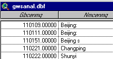
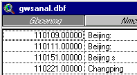
- Click on the column label that says "Gbcenmg" (it's the field with county ID numbers):
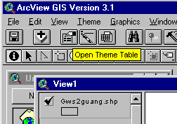
- Now click on the map to go back to the View window and click the "Open Theme Table" button:
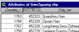
- You'll see the Table for your county. Find the column called "Code_9071" and click the column label
- You'll see that the JOIN button (
 ) lights/becomes un-grey. Click on that button and (if all is well) the data from the gwsanal.dbf will be added onto the end of the Theme Table. Check to see that that's the case (the last column should be labeled "A10409").
- Now from the File menu choose SAVE PROJECT AS,
be sure to put it into your /anth/ folder,
and name it "allgwsjoin.apr"
Now you can explore some of those Analytical Variables (the key is at miley.wlu.edu/gis/easia/analytical1990.html) for your province, by choosing "Graduated Color" as the Legend Type in the Legend Editor window (go back to the second exercise for instructions if you're unsure what to do here).
Try A10155 (sex ratio of population 0-4) {and N.B. that the new variables aren't in numerical order...):

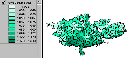
and A10371 (sex ratio of births, 1 Jan '89-30 Jun '90): 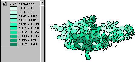
You'd expect these to be pretty similar --but what was the pattern like a decade earlier, and is it any different in its outlines?
The sex ratio of those 10-14 in 1990:
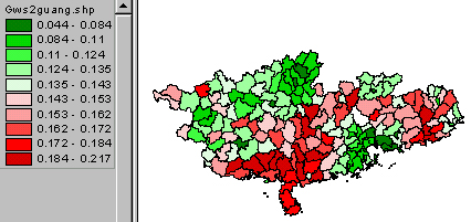
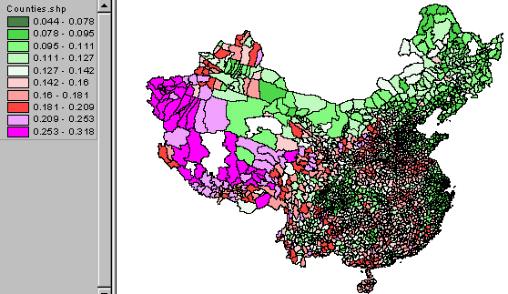
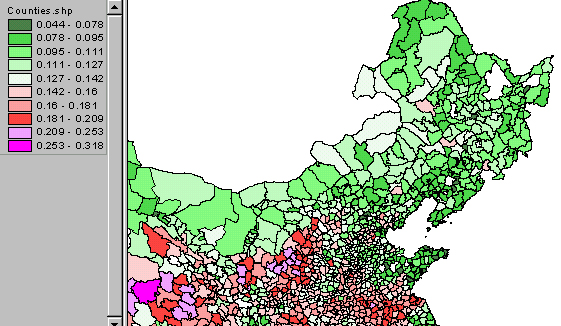
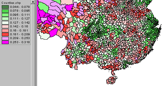
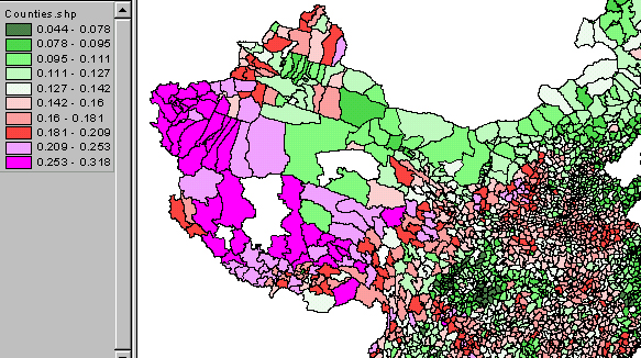
Look at the END of the available variables and find one labeled "bpw" and map that for your Province. It's an Analytical Variable I created to express something of the level of fertility in counties. I added up the number of women in cohorts of childbearing age (a195 + a198 + a201 + a204 + a207 + a210 --those between 15 and 44 in 1990). I then divided the number of births between Jan 1989 and June 1990 (a321) by that sum of "women-at-risk" to get an index of "births per woman", which by itself is probably nonsensical, but produces an interesting distribution. See the overall pattern and zooms for northeast and southeast and west. Your maps of the bpw variable will display variability within your province, so they won't look the same as the overall... but what you should note is: which counties are at the extremes, with either [relatively] high or low bpw? And WHY? My two provinces make an interesting comparison with the images above: